Today, most photovoltaic (PV) renewable energy generation uses solar panels whose PV cells convert sunlight that falls directly on them into electricity. A different approach -- called concentrating photovoltaics (CPV) -- uses optics to concentrate sunlight onto relatively small PV cells which convert that much more intense solar energy into electricity.
Two key performance measures of PV panels are efficiency -- how much power is produced per unit of area -- and economy -- how much power is produced per unit of equipment cost. Conventional PV panels have a well-researched, -understood, and -optimized set of design variables determining such performance characteristics, which can be measured with precision. The same is not true of CPV systems, which have a much larger set of performance-determining variables, and whose efficiency is less easily quantified. The more significant such variables unique to CPV systems include:
The present analysis first establishes a framework for measuring and comparing the area efficiency of all types of PV systems. It then considers the contribution of the last of the above four variables to area efficiency, which is considerable for most CPV systems. The tool GapTrack is used to compare the light-capture efficiency of selected CPV array geometries, including that of ArcSolTM.
The light-capture efficiency of arrays of tracking elements can be computed using CAD models such as GapTrack and can be combined with nameplate module efficiencies and tracker load estimates to compute estimates of array area efficiencies. With this method, the system efficiencies of PV and CPV arrays can be modeled and compared using a consistent metric.
The term module efficiency is used as a specification both of conventional flat-plate PV panels, and of the panel-like modules of CPV systems. This is a source of confusion when comparing the performance of systems of the two types, not only because the solar resource available to CPV is less, but alsobecause the relationship of module efficiency to system efficiency is different in the two cases.
In both cases, module efficiency measures the ratio of the module's electrical output to the area of its front side under a set of reference conditions such as Standard Test Conditions (STC), which illuminates the panel to simulate the sun shining on the panel from its normal (perpendicular) axis through clear skies at a mid latitude. In both cases, that reference output is approached when the sun lies on the module's normal axis. However, whereas the output of a flat-plate PV panel falls off gradually as the sun departs from that axis, the output of a typical CPV module falls off drastically when the sun moves as little as a degree from that axis. Because such CPV modules must be mounted to track the sun, systems built of such modules incur several energy transmission losses beyond those in the modules themselves -- losses that reduce system efficiencies considerably below module efficiencies. Two such losses are uncaptured light falling between adjacent modules, and energy demands of the tracking systems.
Module efficiency shouldn't be used to compare the efficiencies of CPV systems to those of conventional PV systems because it represents different parts of the systems' respective efficiency equations. Module efficiency is also of limited value in comparing the performance of different CPV systems because it fails to capture inefficiencies in the tracking optical geometries of CPV arrays.
In contrast, area efficiency can be defined to enable an apples-to-apples comparison of CPV systems to each other, as well as comparison of the efficiencies of CPV to PV systems taking into account the difference in the available solar resource for the two types. The area efficiency of such a system is simply the ratio of the system's nameplate peak electrical output (defined by its modules' cumulative peak output) to its occupied area. The measure scales from the panel to the solar farm, and can be measured with precision for both PV and CPV systems. (Because module efficiency is based on the sun being in the normal direction, area efficiency is somewhat artificial applied to land-based installations in mid-latitudes where the sun never reaches zenith. Nonetheless it provides a consistent comparison metric between the area footprint of different types of solar installations.)
For a tiling (dense-packed) array of plate-type PV panels, the area efficiency of the array is essentially equal to the module efficiency. For an array of tracking CPV elements, the area efficiency is generally far less than the module efficiency and is greatly influenced by the layout of elements in the array. Although some CPV system designs do not specify layouts, their area efficiency can be defined using the densest layout that allows the full range of tracking motion of the individual elements.
The presence of light-capture gaps in CPV arrays that vary as a function of tracking orientation call for an area efficiency function to predict system performance. Such a function describes the efficiency as a function of the sun's sky coordinates. More specifically, the area efficiency function returns, for any sun-position in a two-dimensional span of the sky, the ratio of the system's electrical output to its total aperture, where the aperture is the system's area times the cosine of the sun's zenith angle.
Like its scalar counterpart, the area efficiency function scales from the square meter to the hectare. The area efficiency function of a single panel can be compiled by measuring its output under STC-like-conditions for a series of different positions of the sun relative to the panel's normal axis, where the aperture is the panel's area times the cosine of the light's incidence angle.
The area efficiency function is not very interesting for plate-type panels over low incidence angles. This is because the light transmission properties of the panel's optical interfaces vary only slightly with respect to incidence angle for such angles up to about 40 degrees, so the fraction of light absorbed by the cells remains little changed and the area efficiency function remains relatively flat.
In the case of CPV systems, the area efficiency function is much more interesting, but poorly studied. Many proposed and some existing CPV systems use arrays of regularly-spaced identical tracking CPV elements. The geometry of these arrays -- the shapes of the elements, the shapes of their clearance profiles as they pivot, and their arrangement in regular patterns -- is a critical determinant of their area efficiency. Because of the constraints of their geometric design many such arrays have large gaps in coverage for portions of the sky and some have restricted tracking ranges.
Area efficiency is the product of a series of efficiency factors, each representing a stage -- such as light traversing a material interface -- that absorbs some fraction of the energy passing through it. Arrays of tracking CPV elements require an additional efficiency factor not needed to compute the area efficiency of fixed panel arrays -- that giving the ratio of light entering the array's aperture to that entering an element's aperture.
Since this factor is a function of the sun's position relative to the array, it can be used to define the light-capture efficiency function with respect to the sun's sky coordinates. That function is determined by the geometry of the array -- specifically the shapes of the solar modules themselves and the way in which they pivot on their tracking mounts. That fact prompts the question: Is there an optimal geometry for the CPV array -- one that maximizes the light-capture efficiency over a wide range of 2-axis tracking motion?
Existing CPV array geometries do not show evidence that this question has been answered or even asked. Perhaps this is because most CPV arrays, being bulky land-based installations, are spaced out to maximize equipment utilization -- by avoiding shading of CPV elements by their neighbors for greater portions of the day -- at the expense of area efficiency. In fact, solar farms, whether PV, CPV or CSP-based, tend to have appallingly low area efficiencies.
The importance of an array geometry that optimizes area efficiency becomes clearer when one considers the implications of miniaturizing CPV arrays. Panels encapsulating such arrays could potentially deliver twice as much power as crystalline silicon PV panels having the same footprint, and could be used in the same applications.
The question of whether there is an optimal geometry is more likely to have an answer for the case in which the CPV elements are required to be collision-free regardless of their unsynchronized motion. This non-collision feature is essential in CPV array designs in which the CPV elements are mechanically independent. It is also desirable in some designs that mechanically synchronize the tracking of groups of CPV elements, because the failure of the mechanical interlinkage could leave a CPV element in a position unsynchronized with its neighbors.
The following analysis of optimal array geometries makes these assumptions:
With the addition of the fifth assumption, it may not be obvious that there is a solution:
The foregoing assumptions preclude the use of an altazimuth mount, because a tiling shape cannot be rotated about its normal axis (which corresponds to the azimuth axis when the light-capture components tile) without parts of it deviating outside of its profile. Therefore, a sixth assumption is made that:
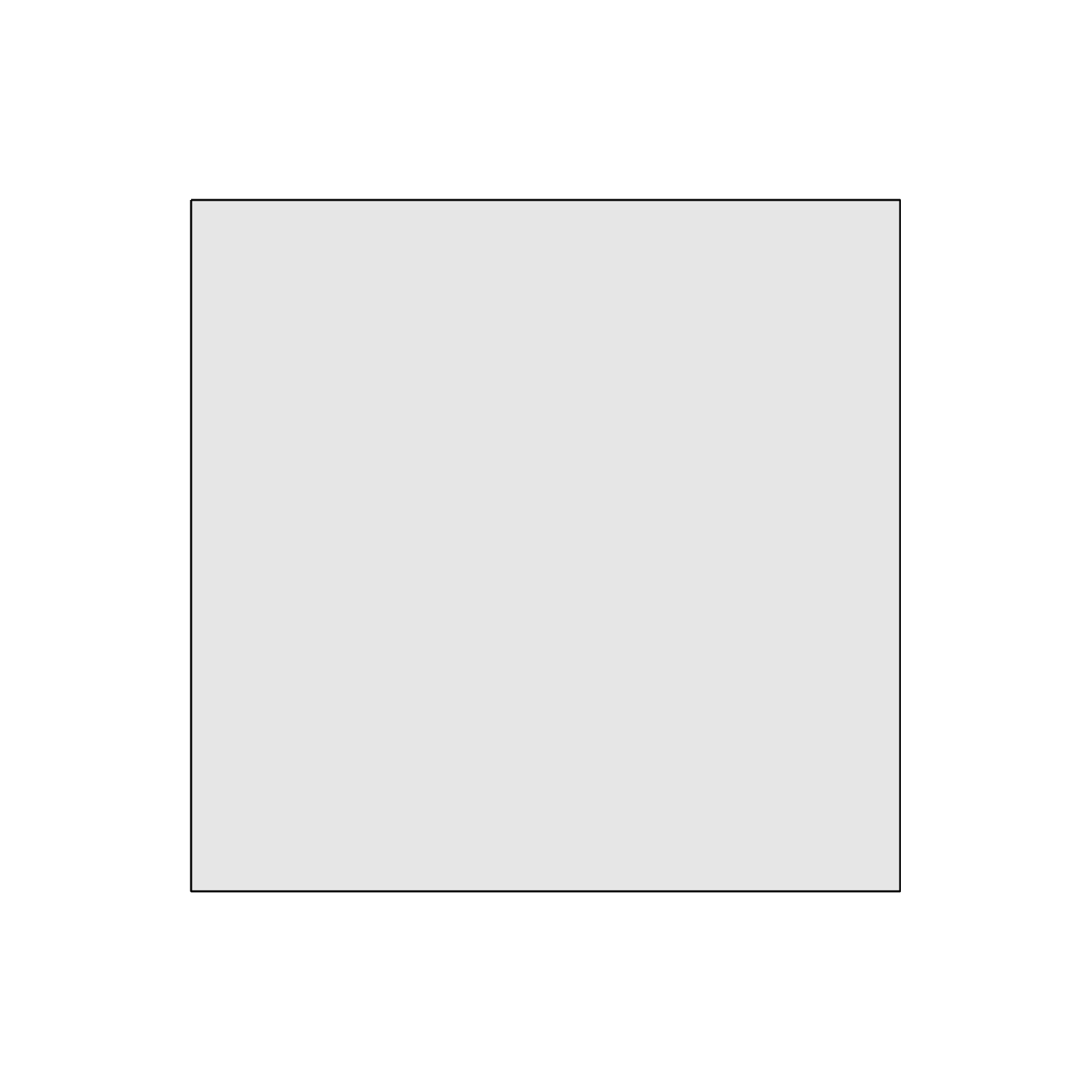
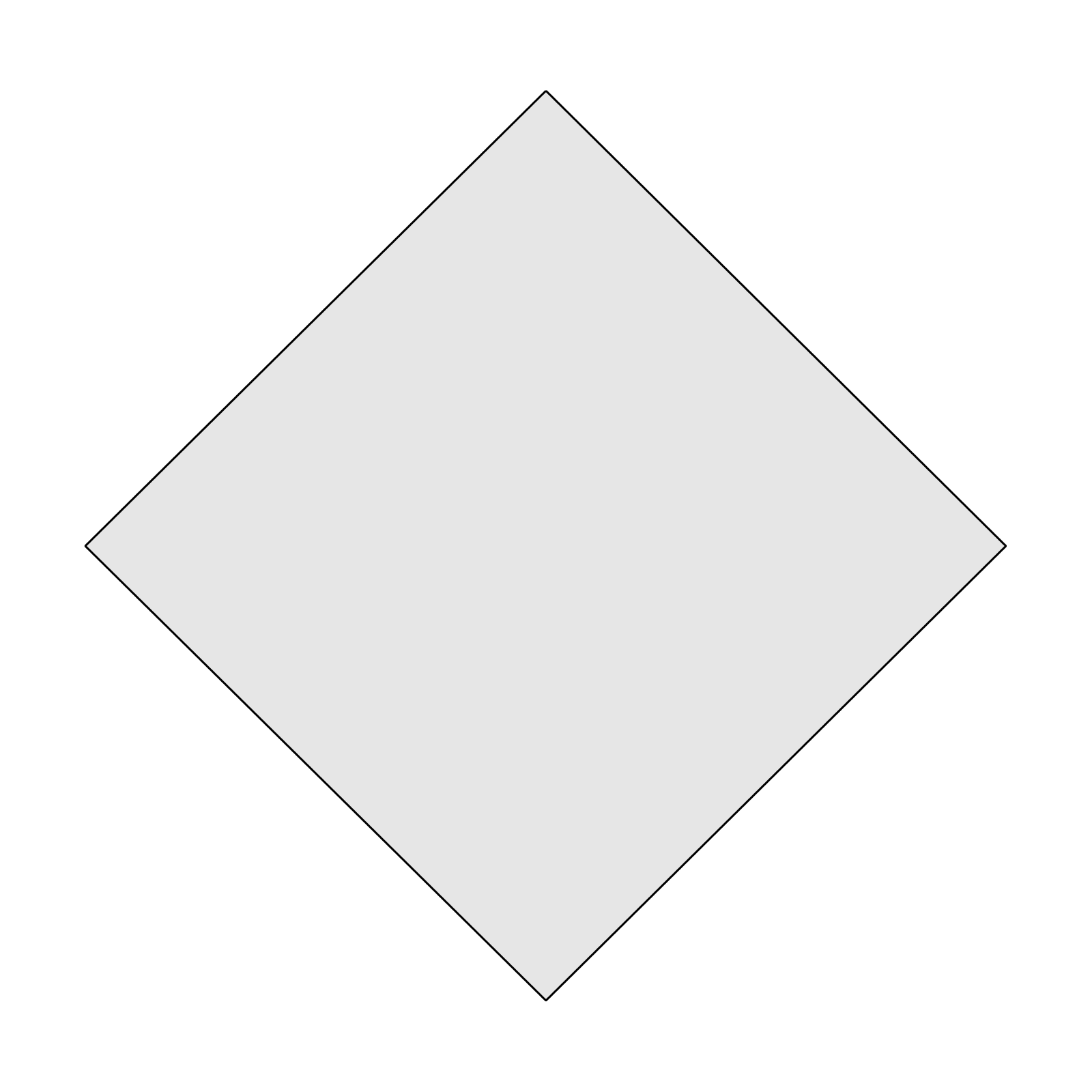
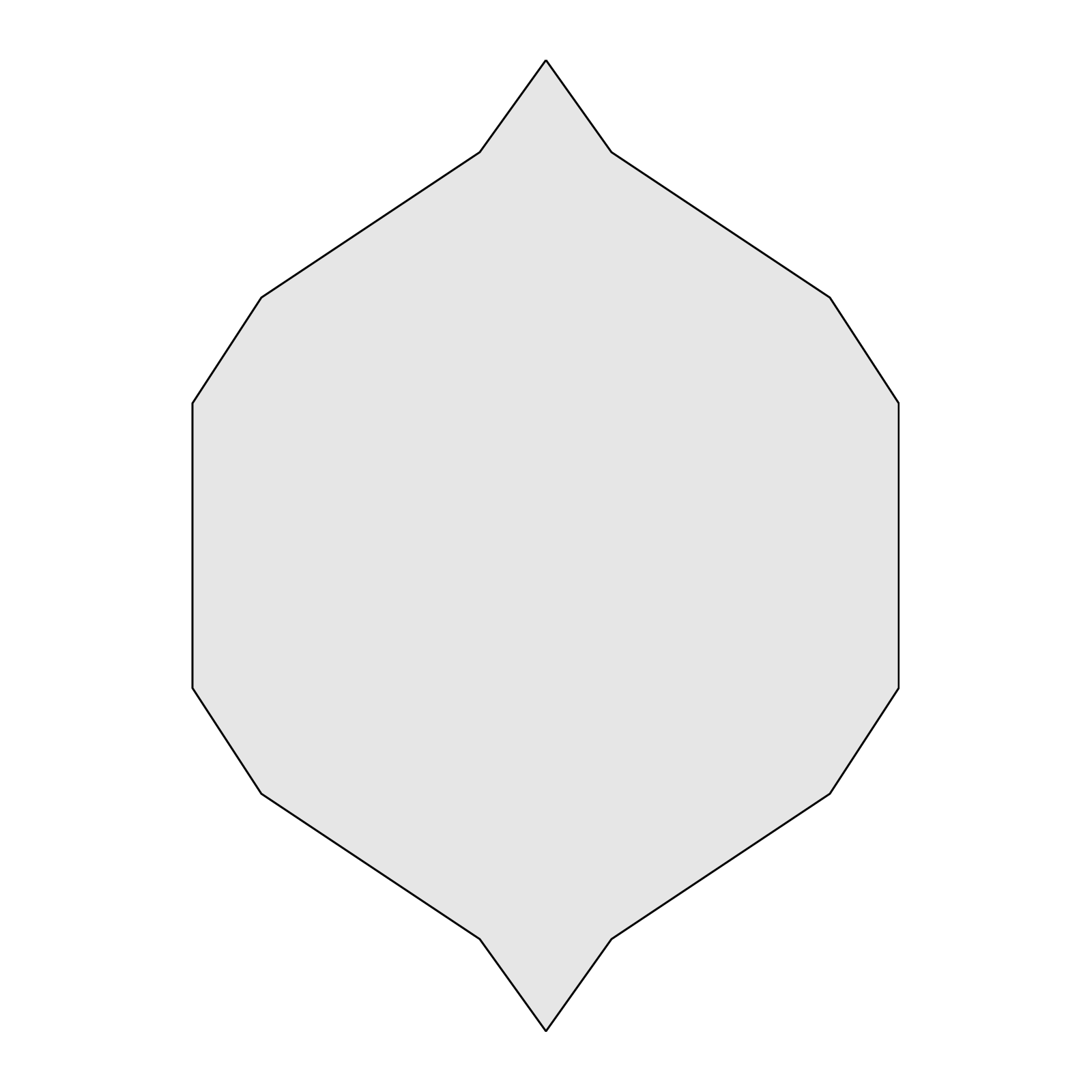
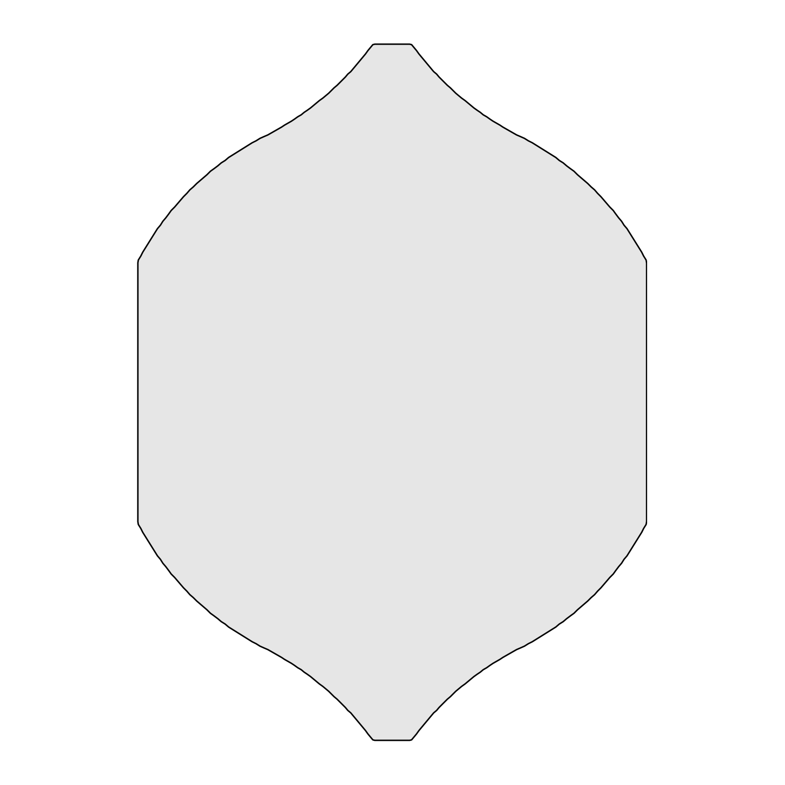
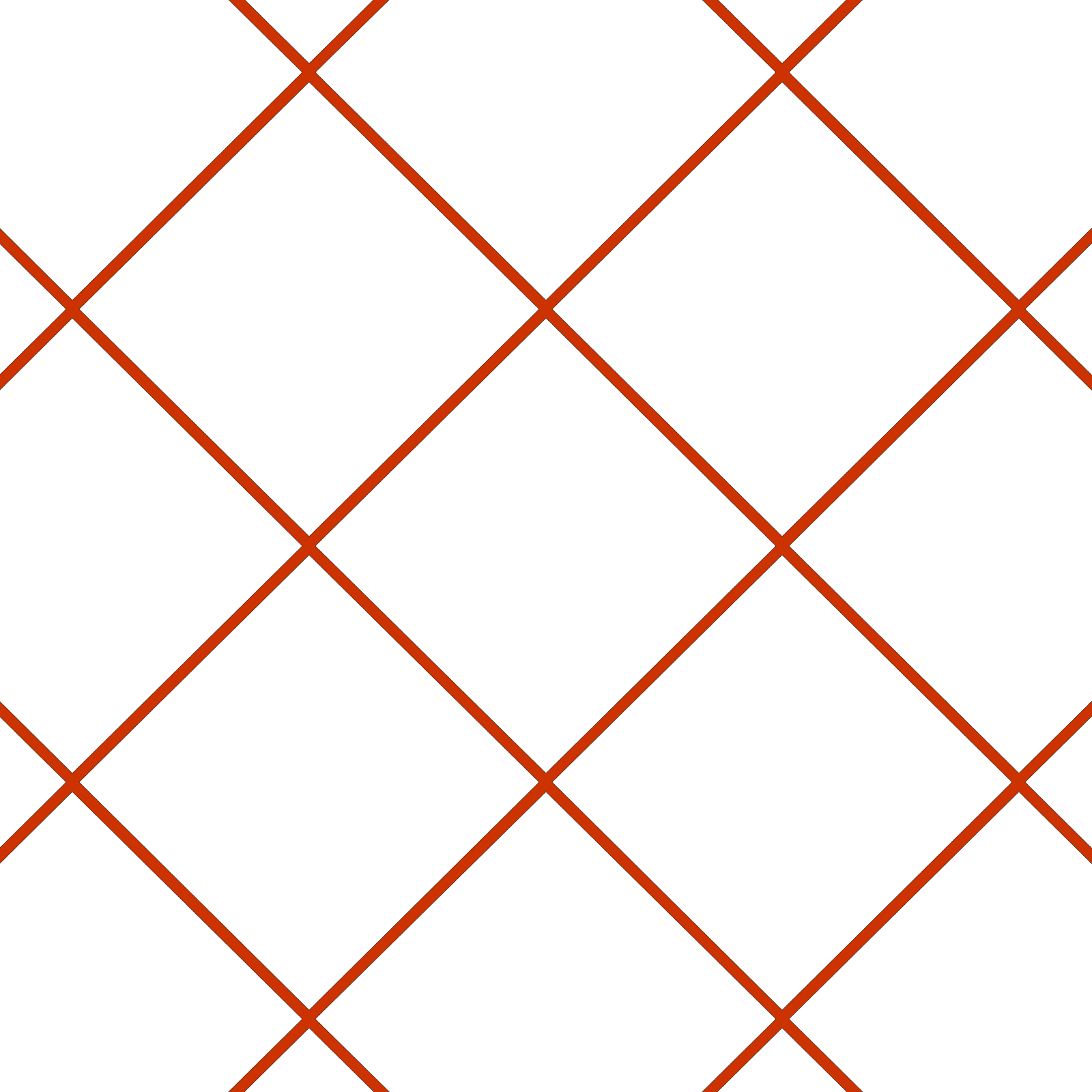
Given these assumptions, tiling shapes can be tested for collision using the simulation tool, GapTrack, designed for this purpose. The following graphic shows five tiling shapes: a square, a diamond, a hexagon, a 14-sided shape with two-fold symmetry, and a similar shape with straight and arcuate edges.
 |
 |
 |
 |
 |
 |
 |
 |
 |
 |
|
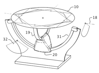
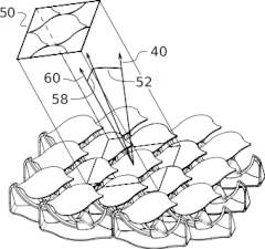
| This illustration from the 'ArcSol' patent application shows a nested two-axis mount that produces the same kind of pivoting motion as a classic double gimbal mount having an outer tilt axis (32) parallel to the base plane, and an inner tilt axis (18) perpendicular to and intersecting the outer axis. The pictured ArcSolTM mount provides this pivoting motion using an angular positioning unit (20) that moves relative to the concave arc (31) and the smaller convex arc (19). |
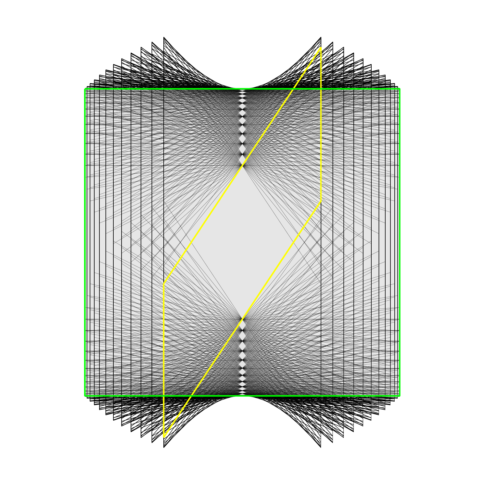
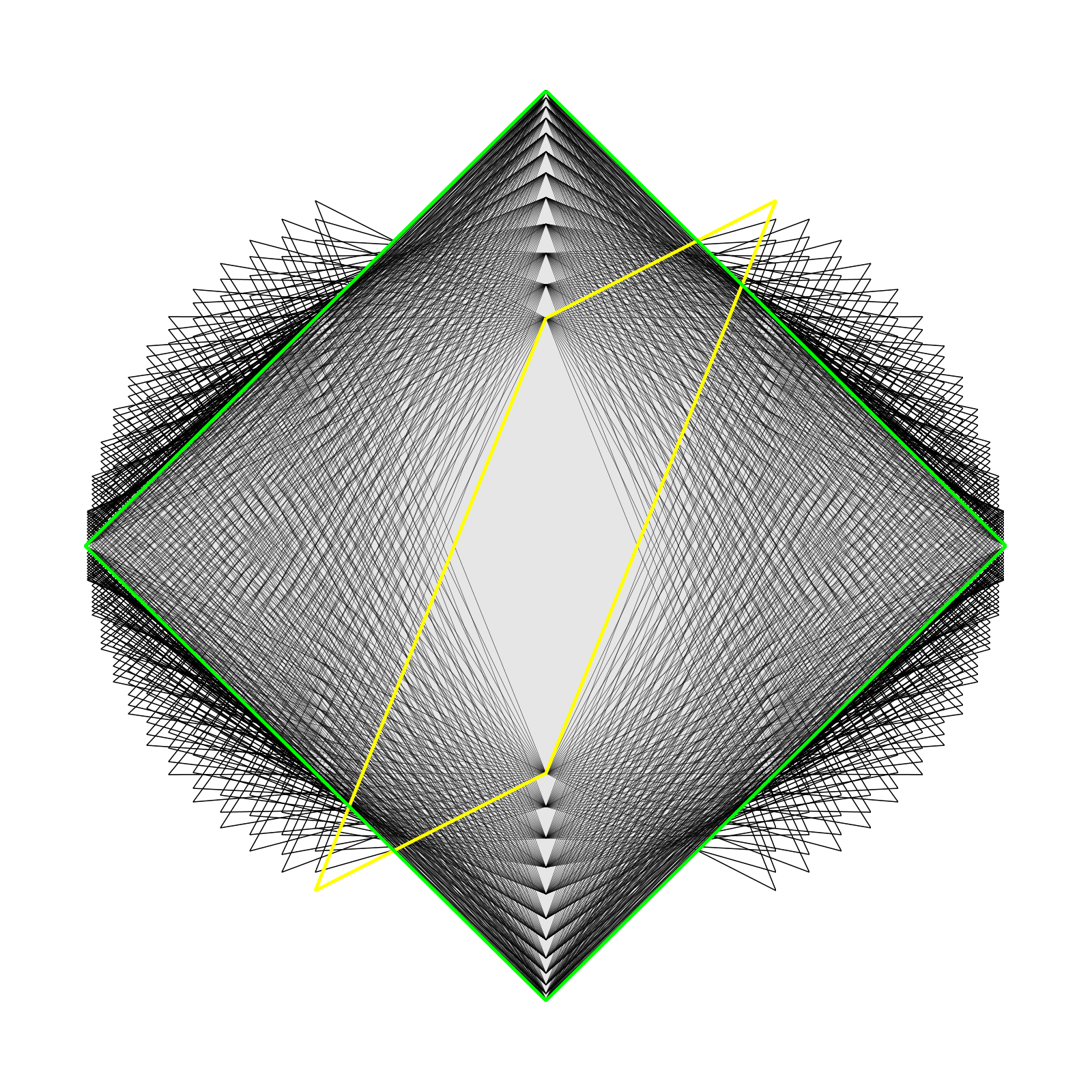
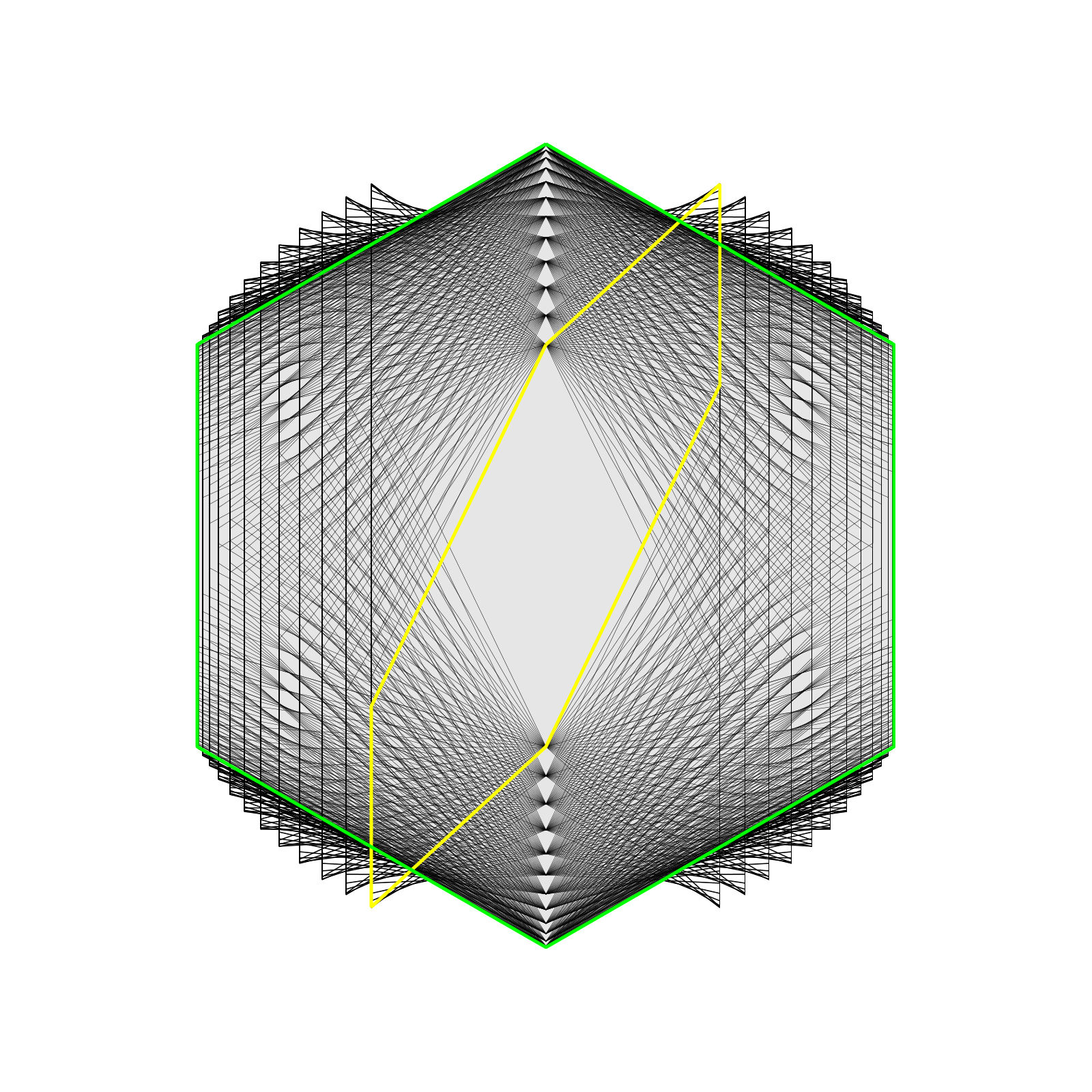
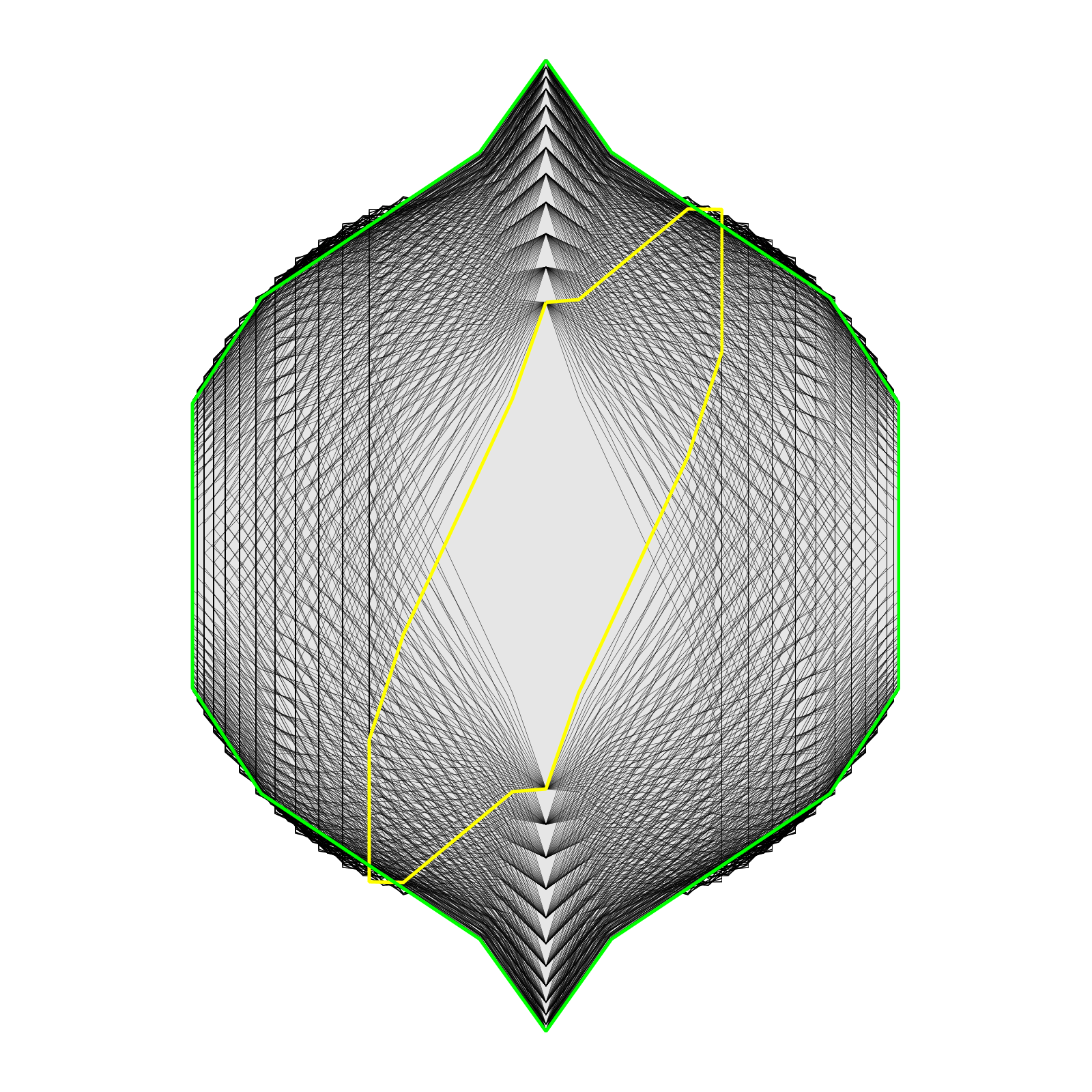
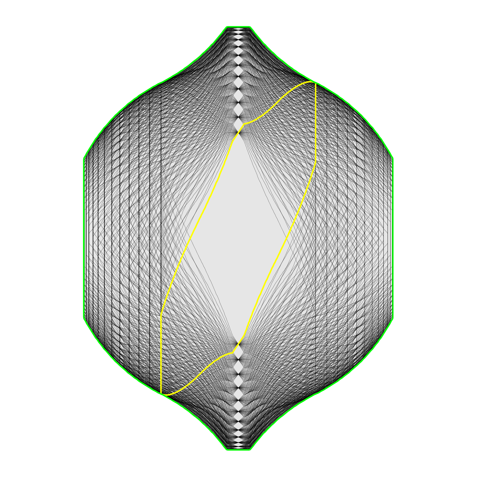
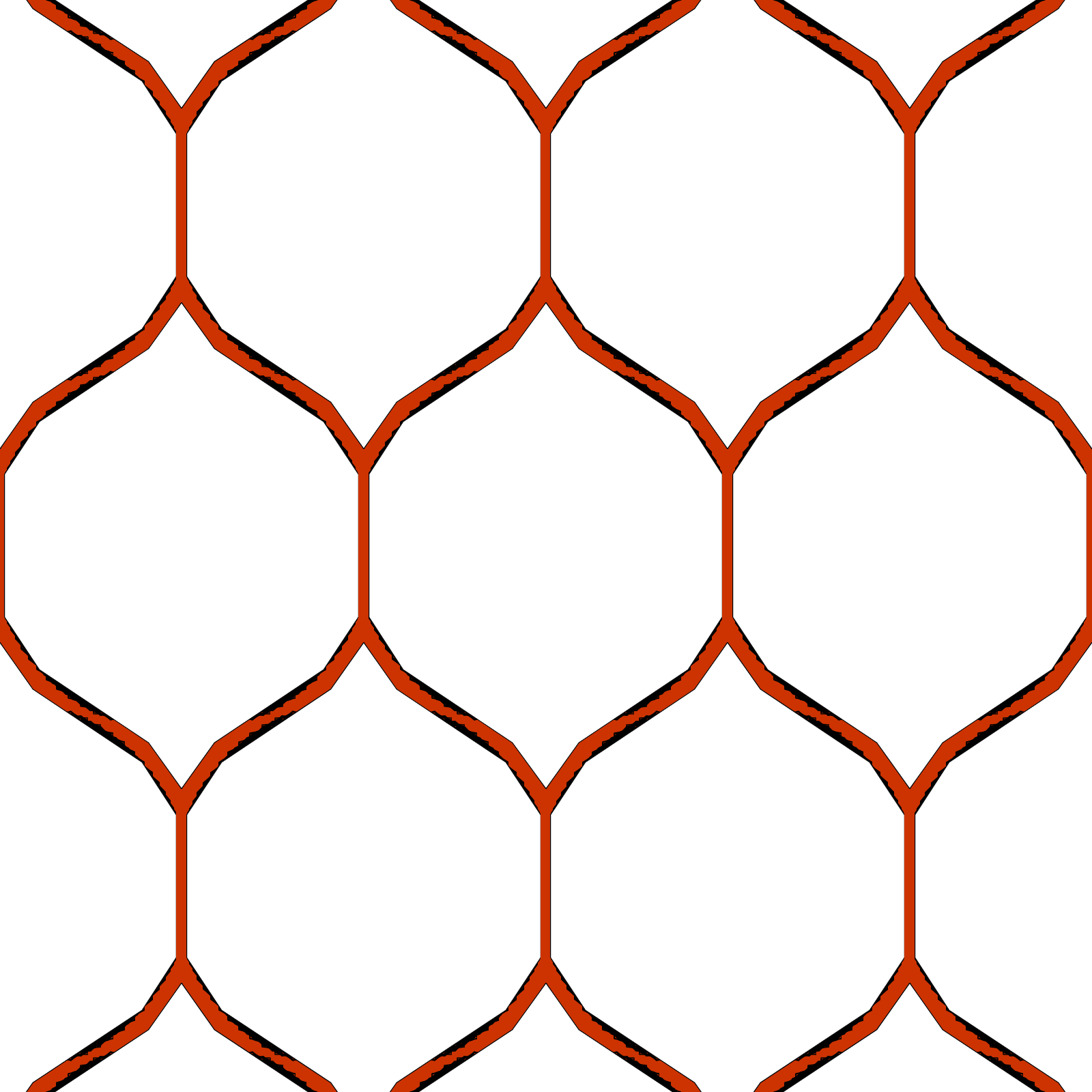
The method of collision testing is illustrated by the figure to the right and the following graphics. The plate (10) is moved through a range of angular motion that takes it up to 60 degrees from normal about both tilt axes. Tiling profiles drawn on the plate are projected onto a plane parallel to the base for each of numerous tilt angles.
The first row of graphics below shows the results for each of the shapes described above. The un-tilted profile is outlined in green, and the tilted profiles are outlined in black, with one tilted 60 degrees about both axes outlined in yellow. For each of the three regular polygons, pivoting generates significant excursions outside of the original profile. The fourth shape generates only minor excursions, and the fifth shape generates none.
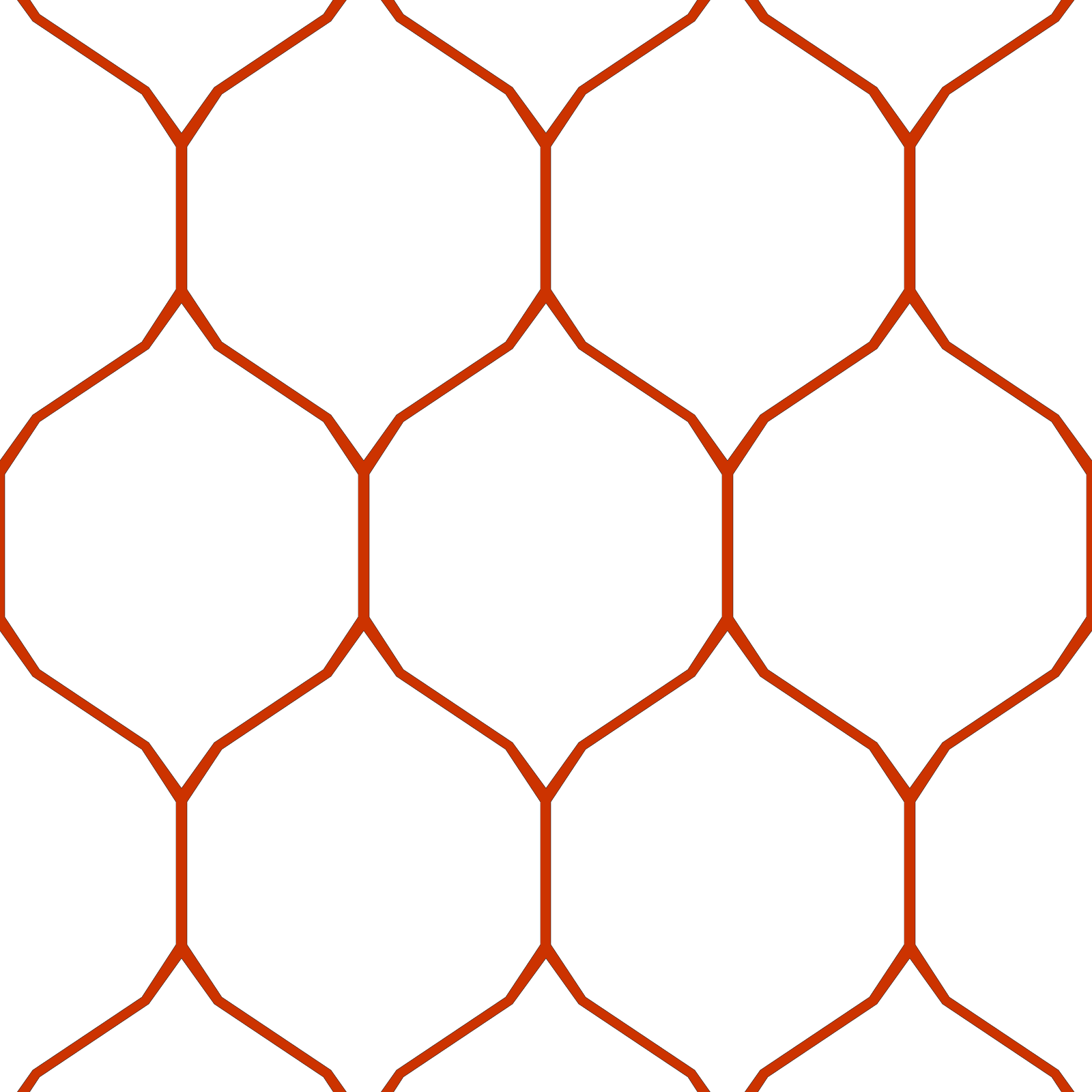
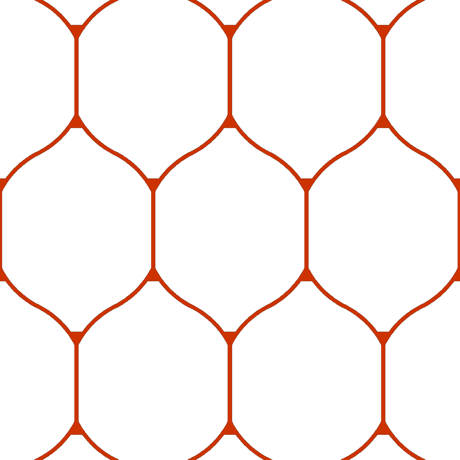
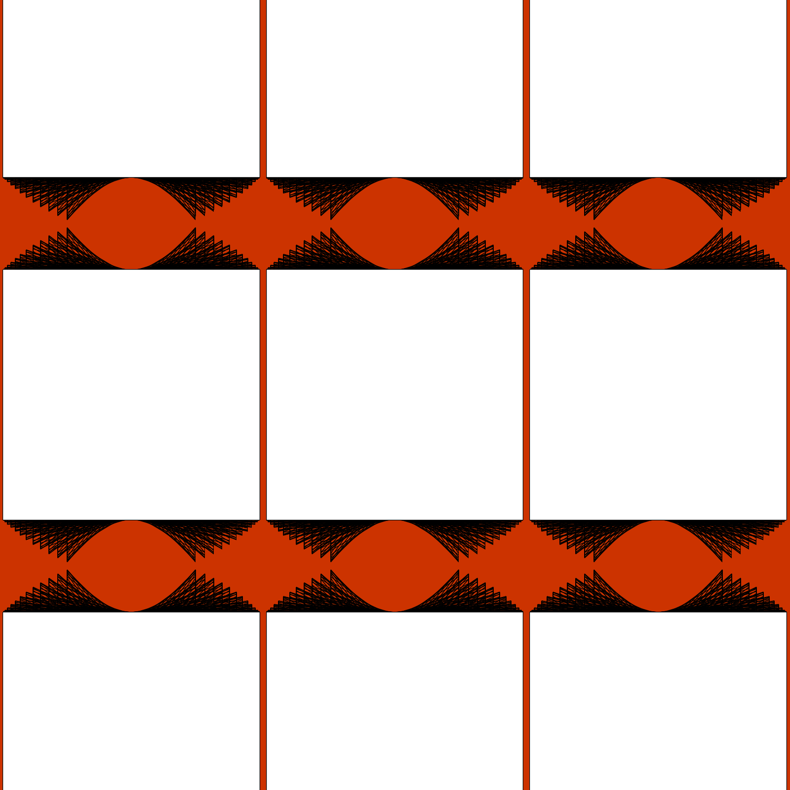
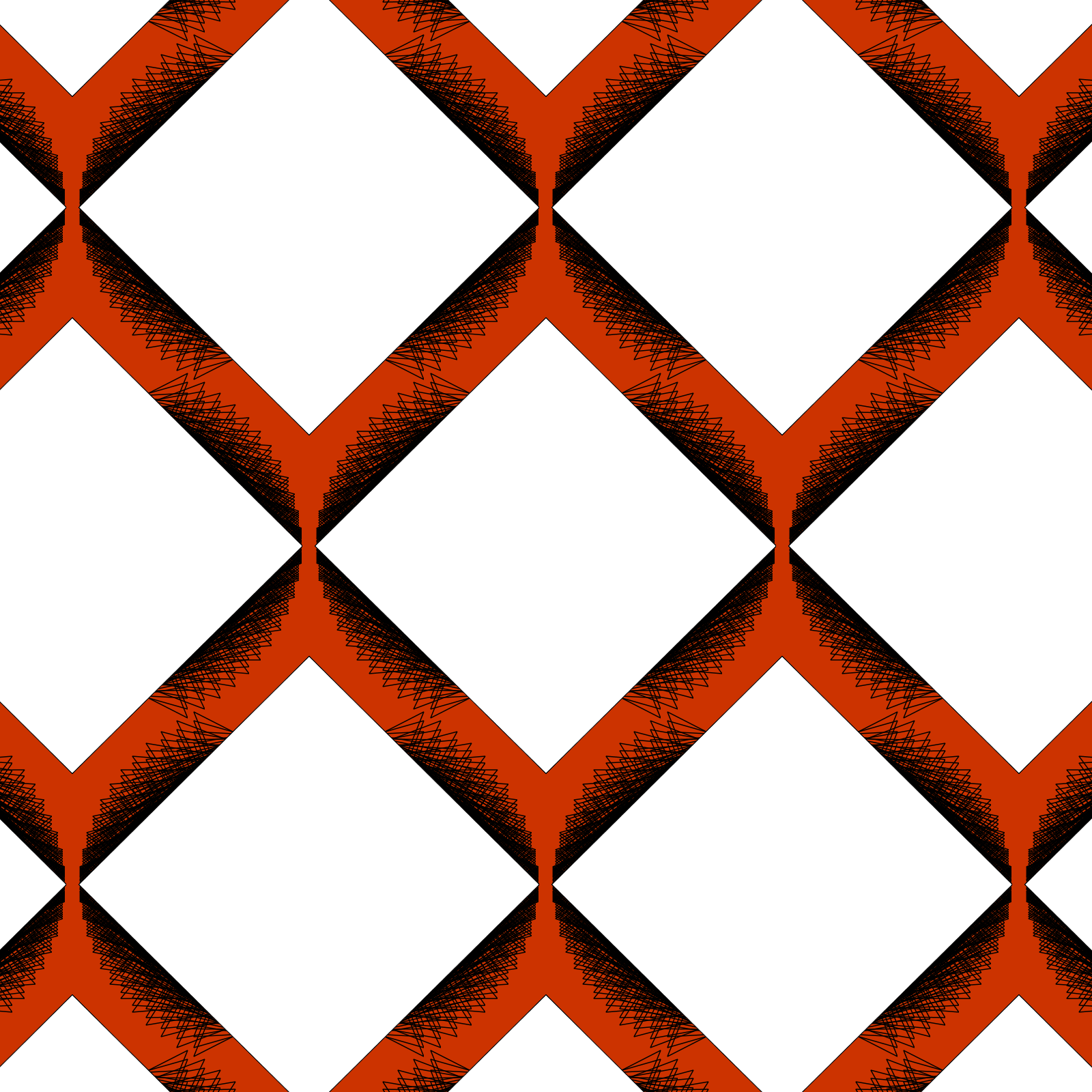
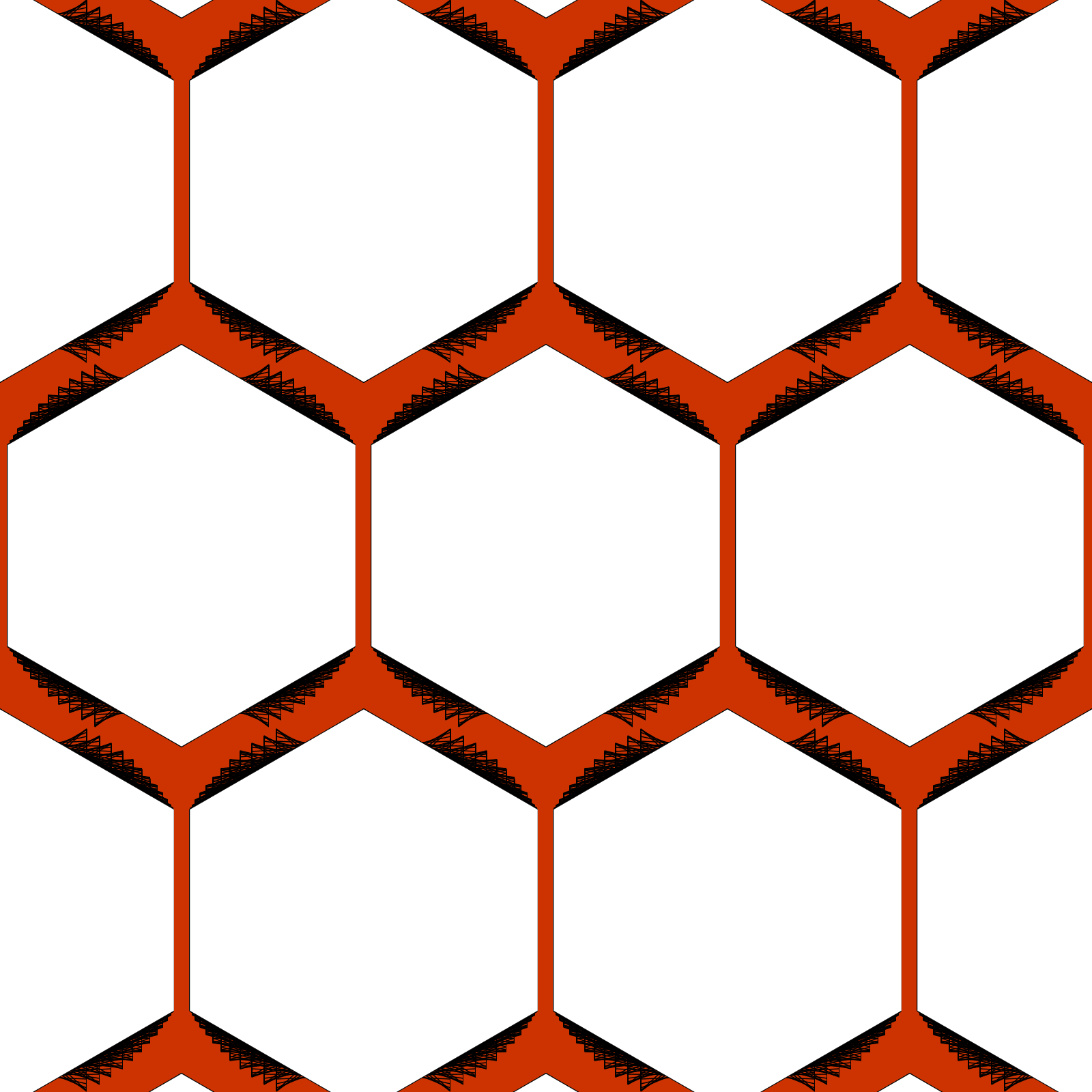
The second row of graphics shows arrays for the respective shapes, where buffer spacing has been added to eliminate the possibility of collision.
 |
 |
 |
 |
 |
 |
 |
 |
 |
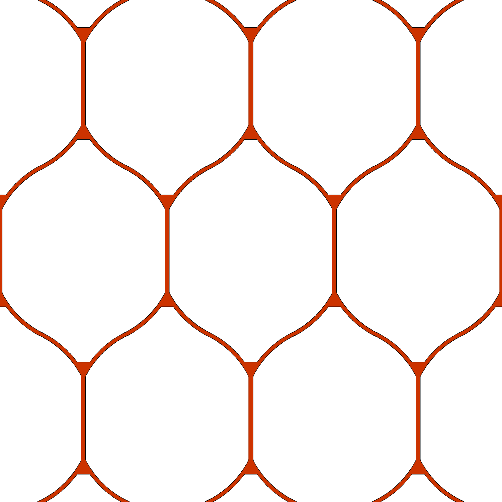 |
In the case of the square, diamond and hexagon, the spacing required to preclude collisions costs the light-capture efficiency between 25 and 30 percent when the sun is in the array's normal position. In contrast, the 14-sided shape loses about five percent, and the fifth shape loses none to such required added spacing and loses about three percent to the default inter-tile spacing.
|
| GapTrack simulates sun's-eye views (50) of a small region of an array of light-capture elements over a range of tilt angles. The sun lies on the center element's normal axis (60), which is tilted away from the array's normal axis (40) by the outer-axis tilt angle (52) and the innter-axis tilt angle (58). |
Light-capture efficiency for array-normal incident light is important, but what does that efficiency look like over the useful range of tilt angles for the various shapes? GapTrack answers this question by simulating the sun's view of a portion an array for a given pair of tilt angles. For a given shape, the first step is to generate a matrix of light-coverage images whose columns and rows correspond to five-degree increments in the inner-axis and outer-axis tilt angles, respectively.
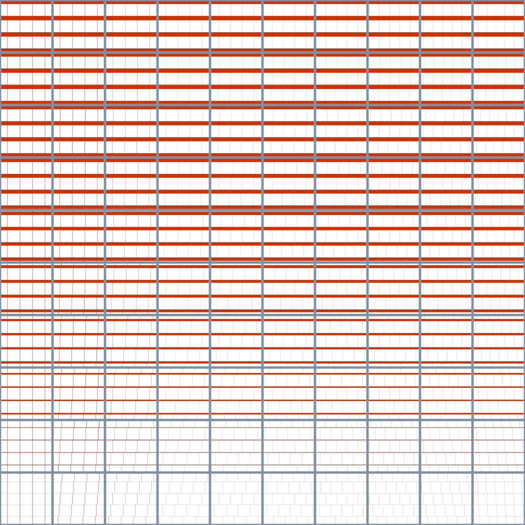
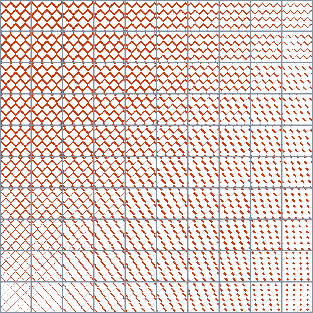
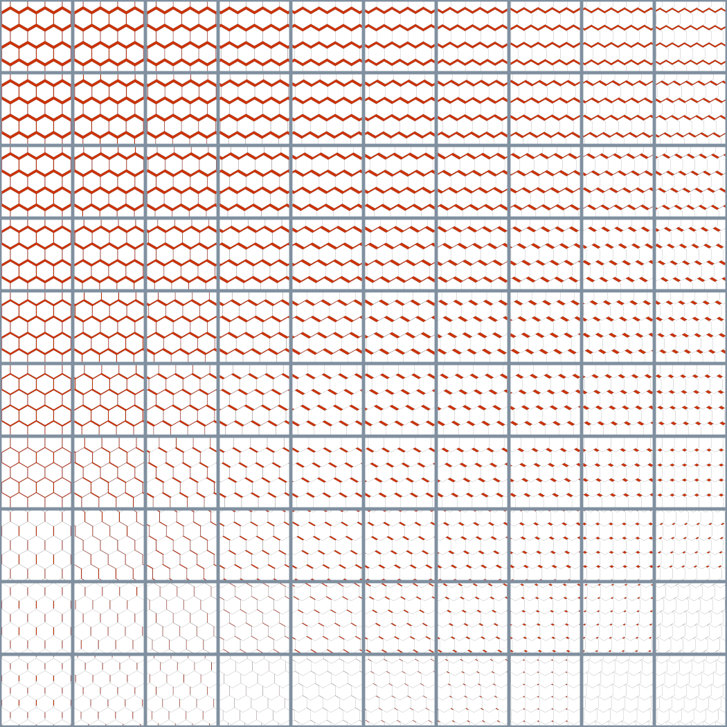
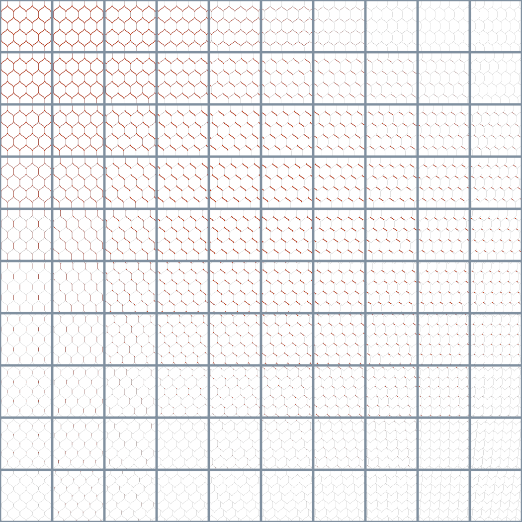
Such a tilt-angle matrix is shown for each of the five shapes below, where the light-capture gaps are shown in red. In each case the inner-axis angle increases from left to right and the outer-axis angle increases from top to bottom. Thus, the upper-left cell corresponds to tilts of zero, and the right column and bottom row correspond respectively to inner- and outer-axis rotations of 45 degrees.
 |
 |
 |
 |
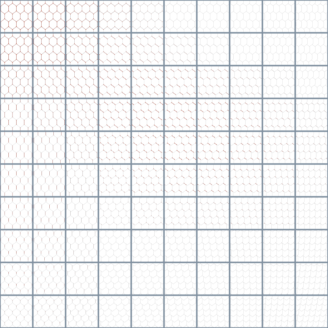 |
In general, the light-capture efficiency increases as tilt angles increase, because the greater overlap of the shapes at higher tilt angles tends to reduce light-capture gaps. However, the central peak in inefficiency tends to make a broad plateau extending out to tilt angles of about 25 degrees and more.
|
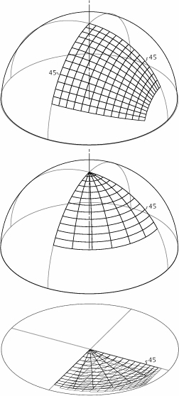
| One quadrant of angular position space as a grid mapped to the upper hemisphere (top); The spherical coordinate system as a grid covering part of the same upper hemisphere quadrant (middle); and projections of the two grids to a quadrant of the disk (bottom). |
GapTrack measures the capture efficiency of a cell in the tilt-angle matrix by histogramming its image and quantifying the relative area of the gap-signifying red. It can graph the efficiency over the Cartesian coordinate system of inner and outer tilt angles. Such a graph would be misleading in quantifying overall efficiency because some parts of the tilt-angle space are more important to efficiency than others. Cells in a tilt-angle graph neither represent equal areas of sky coverage nor do they take into account that the array's aperture varies with light's incidence angle on it. What's needed is a map of the capture efficiency in which equal areas approximate equal maximum energy flux on the array's aperture.
GapTrack provides the needed energy-flow-normalized representation, where tilt-angle coordinates are mapped to spherical coordinates, and then projected onto the disk. An inverse operation recovers tilt angles from disk coordinates. In the disk, equal areas represent equal aggregate apertures, because the scaling of regions of the hemisphere projected onto the disk is proportional to the sine of the elevation angle (ninety degrees minus the incidence angle) in the same way that the aperture varies with the sine of the elevation angle due to foreshortening of the array's footprint.
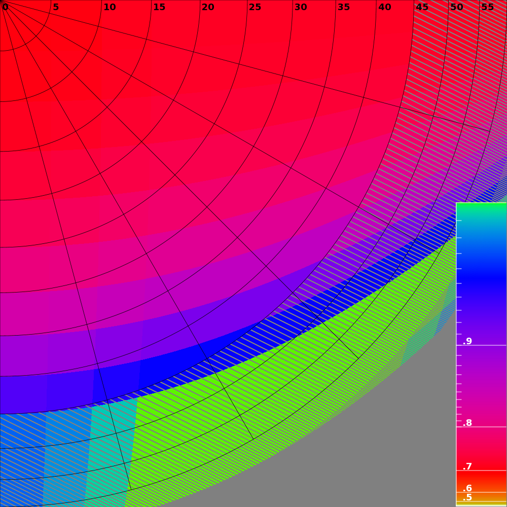
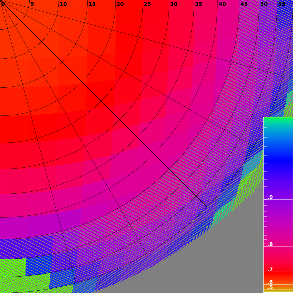
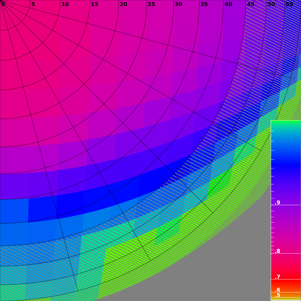
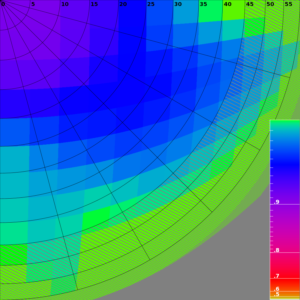
The images below are graphs of capture efficiency over a quadrant of the disk for the same tiling shapes shown above. Efficiency is indicated by color, which is green for one hundred percent. The graphs shade areas whose incidence angle is greater than 45 degrees, to indicate increasing losses -- other than due to aperture foreshortening -- that begin to become significant thereabout.
 |
 |
 |
 |
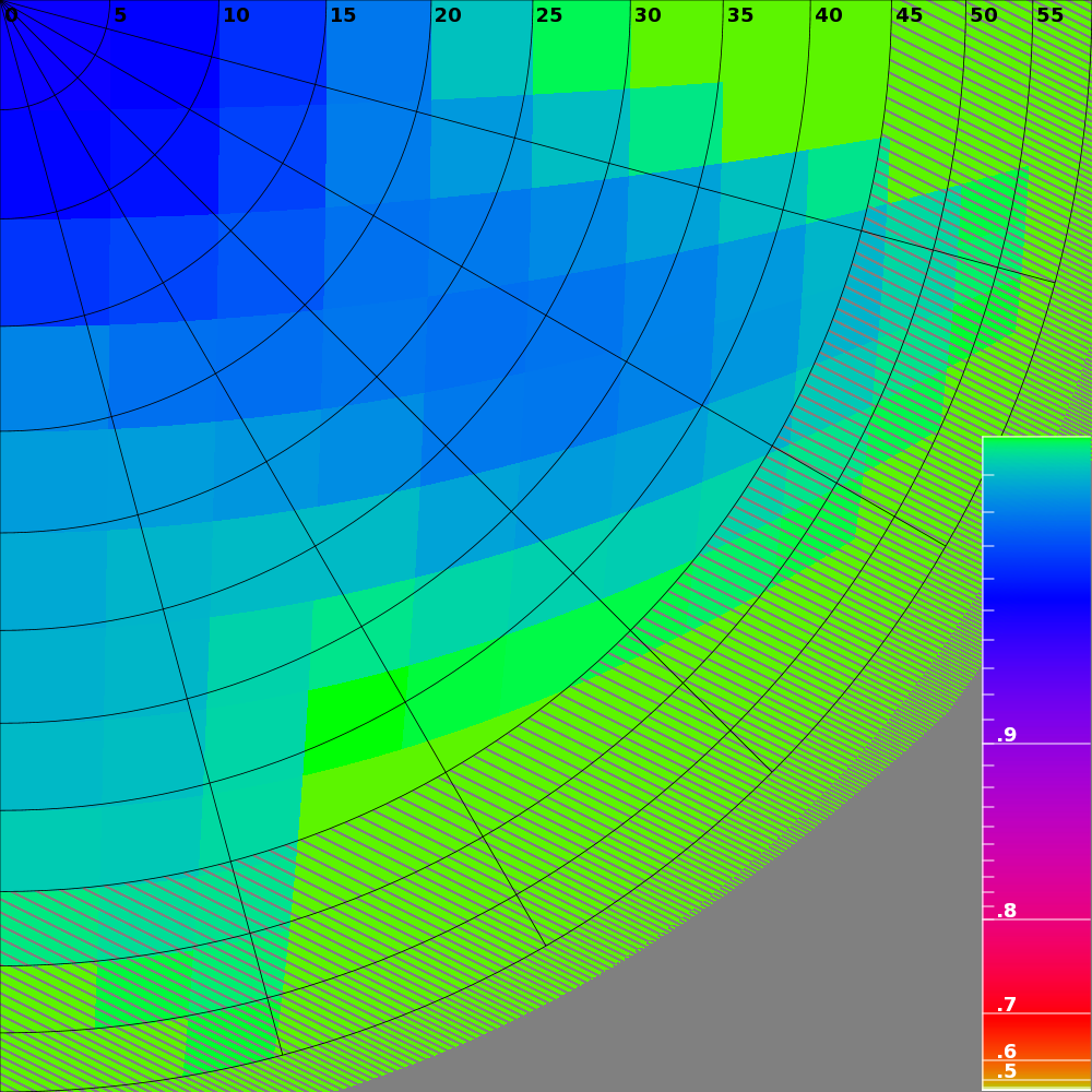 |
The graphs show 25 to 30 percent losses in light-capture efficiency of tracking arrays of regular polygons extends over much of their useful tracking range. In contrast, the ArcSol shape loses less than 4 percent anywhere in that range, with the largest losses occurring near the normal angle.
A definition of area efficiency, and of a related area efficiency function over the range of light incidence angles, allows the power densities of all types of solar electricity generation systems to be compared -- from fixed and tracked PV systems to externally and internally tracked CPV systems.
The two largest factors in determining the area efficiency of a tracked CPV array are the module efficiencies of the array elements, and the the light-capture efficiency of the array, where the latter describes the likelihood that light falling within an array will be captured by a module belonging to an array element. Thus, light-capture efficiency quantifies losses before light reaches a module's face, and module efficiency quantifies losses from that point until the light is converted to electricity. Although module efficiency is established through testing under standard conditions and is typically included in product specifications, the light-capture efficiency is not commonly addressed. Fortunately, light-capture efficiency can be computed over the range of light incidence angles given a geometric model of the array, and can be used, in conjunction with known module efficiencies, to accurately estimate the area efficiency of proposed installations.
The tool GapTrack was used to compute the light-capture efficiency functions for several plane-tiling shapes supported on two-axis mounts that pivot the shapes about their centers. Simple plane-tiling shapes require the addition of buffer spacing between adjacent elements to preclude collisions, costing up to 30 percent of light-capture efficiency. In contrast, the ArcSol shape sweeps out a volume that is circumscribed by the shape's profile, and therefore requires no such buffer spacing. It achieves nearly perfect light-capture efficiencies over the entire range of incidence angles.